BUFKIT is an analysis tool kit, and it’s used by forecasters to better understand what is happening with the atmosphere by looking at it vertically. It’s a widely used tool, from forecasters in the National Weather Service to hobbyists, and looks great on resumes for those meteorology students who wish to go into an operational forecasting position.

DISCLAIMER

This is for BUFKIT 2017. This article may not be updated for any future versions.

Downloading

If you haven’t download BUFKIT, you can download it here (direct download) and go through the installation process. Once you have it installed, open it up.

Interface: Part 1

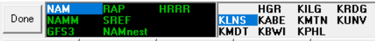
In the top left, there is a “Done” button, along some text. The text in green are your models, while the text all the way on the right are the station identifiers. These are your stations that you have data imported for (we will discuss importing data later). Here, I have KLNS (Lancaster, PA), HGR (Hagerstown, MD), and a few others. You can have as many as you’d like here. The “Done” button is the equivalent of clicking the fancy red “x” in the upper right corner.

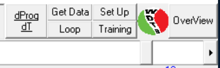
Now, let’s discuss what’s going on in the upper right corner.
Get Data: This button allows you to get the BUFKIT profiles you want. We will discuss this in detail a bit later.
Set Up: If you click this, a pop up window will appear with a few settings. The only thing you should modify for the time being is the timezone. Once you do that, hit “save”, and the window will automatically close.
Loop: This button loops the skew-t. The settings for this can be found under the “controls” button (which is explained later).
Training: Utilize this. The training button opens up a new window and gives you a thorough run-through of what BUFKIT is and provides a few forecasting techniques that go hand-in hand with using the software.
Overview: I won’t get into detail with what this is here (future blog TBD), but you’re looking at how a parameter or variable progresses with time and height (such as temperature, dewpoint), with the current time being highlighted with a vertical white line. Go ahead and play around with this and see what you discover with it.
dProg/dT: If you have past model data archived, you can view the data and compare it to the current model run using dProg/dT.

Getting the Data

Getting the data is very easy and somewhat straight forward. Go ahead and click on the “Get Data” tab. A new window will open (Note: this is called BufGet). If you go most of the way down in the window, you’ll see an area called “Load Profile List”. Go ahead and select the letter C. You can type in the black area, so go ahead and highlight everything in the black area and delete it. Go to one of these websites (or both if you wish):

1. Penn State Bufkit
2. Iowa State Bufkit

Before continuing, I want to make mention that not every point on either site has model data available. You may need to pick and choose a different site depending upon what model you want to use.

PENN STATE LINK: On the left side, you will see all the models .buf files they provide, along with each run time. The current model run is highlighted in green (this is what you want to choose). Go ahead and select the latest GFS model run. A new map will quickly load. Click on any station you’d like to. You’ll find yourself on a page with what seems like nonsense, which is what you want. Take note of the URL (be sure it ends in .buf).
IOWA STATE LINK: Scroll down a little bit until you see a map. This map is interactive, unlike the Penn State map. Click on any dot you’d like to get a window to pop open. From there, go ahead and click on the most GFS run (if it’s available – if not, find another station). Now, you should be on a page with what looks like nonsense. Take note of the URL (be sure it ends in .buf)

Go up to the URL and copy it and then open BufGet. Now, let’s archive our data (because it’s always a great idea to archive it) by typing in “Archive on” (without the quotes). Hit enter twice. Now, paste that URL you copied not too long ago. Do note that “Archive on” should be highlighted in red. Yours should look similar to the picture below:

If yours looks like this, you’ve done all the steps correctly thus far! On the right side, click the red letter C under “save profile list”. This is saves your list. Make sure you do this if you’re loading in new profiles. Click “Get Profiles” and let it load in all the profiles. A message will appear saying “Profile List Completed” at the bottom of the window. Now, click Bufkit and you should have the latest profile loaded into BUFKIT for your selected city! Go up to the top and select the model run you just loaded in.

Interface: Part 2

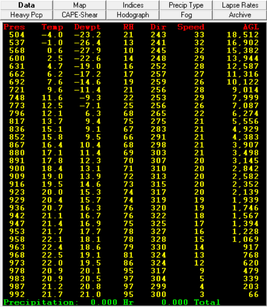
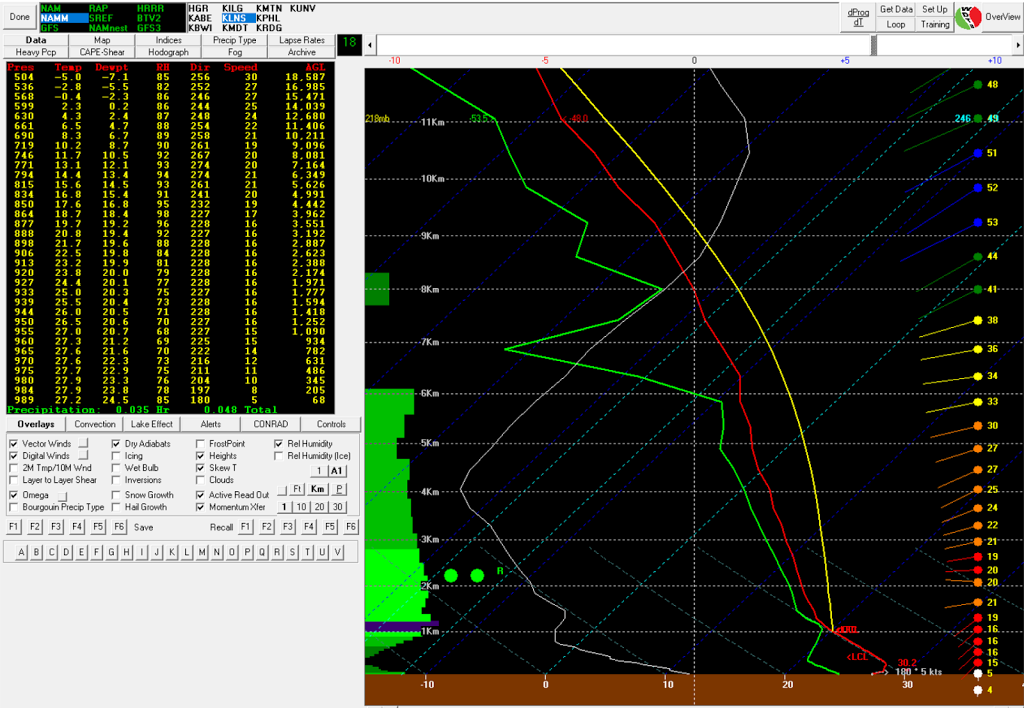
• Data: Starting with the top portion, you should see a lot of yellow numbers. These values are your pressure, temperature (in Celsius), dewpoint (in Celsius), relative humidity, wind direction, speed (in knots), and “above ground level” (in feet). They are numerical values as opposed to the skew-t, and sometimes are easier to read.
• Map: This shows you a map of all the stations you have imported. Go ahead and import another station in a different location by following the steps above this section. You will see another dot appear on this map. You can click these dots to quickly navigate to another station as opposed to finding the station identifier above this section.
• Indices: This shows you your different indices such as CAPE, CIN, K-Index, etc.
• Precip Type: It’s a bit complicated to explain, but the tab says it all: it shows the precipitation type. Once you begin using BUFKIT often, you’ll understand this tab better.
• Lapse Rates: The tab says it all!
• Heavy Pcp: Just like Precip Type, the more you use BUFKIT, the better you will understand it. Don’t worry about it for now.
• CAPE-Shear: This is a plot of shear (x-axis) vs CAPE (y-axis). Just like before, don’t worry about it much for now.
• Hodograph: If you know how to use a hodograph, this is the tab for you! Hodographs are plots of the wind speed and direction.
• Fog: Just like before, don’t worry about it. This is used primarily for fog formation.
• Archive: Remember that “Archive on” I had you type when you were getting data? This is where it’s stored – you can go back and grab any archived skew-t.

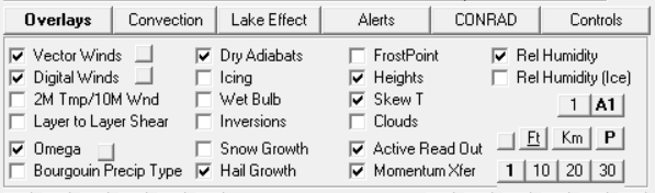
• Overlays: I would suggest you check what I have checked, as I found this setup to be the most useful during the summer months. Everything should be fairly self explanatory, except the “Momentum Xfer” setting. Momentum transfer occurs when the temperatures go up the dry adiabat to bring down the winds from a certain level (normally around 850mb). Generally, 75% of the winds mix down and reach the surface.
• Convection: This tab allows you to display the LFC, LCL, CAPE, Convective Temperature, Elevated Cape and more on the skew-t.
• Lake Effect: This tab is primarily used when the lakes are “turned on” for lake effect snow season.
• Alerts: I’ll be honest – I never use this tab, so I don’t know what it is. CONRAD: Same thing as the alerts tab – I don’t use it, so I don’t know what it is. (Fun tidbit: click on the button that says “Don’t click”.)
• Controls: This allows you to choose your frame speed when you loop the sounding, along with screenshot and export the sounding.

The only way that you will get better with this tool is if you use it. Play around with the different buttons and see what they do and get comfortable with it.